# SCAD thresholding operator: solves the one-variable penalized problem
scad_threshold <- function(z, lambda, a = 3.7) {
  az <- abs(z)
  if (az <= 2 * lambda) {
    sign(z) * max(az - lambda, 0) # soft-threshold region
  } else if (az <= a * lambda) {
    ((a - 1) * z - sign(z) * a * lambda) / (a - 2)# linear middle region
  } else {
    z # no shrinkage
  }
}The SCAD Penalty for High-Dimensional Regression
Statistics
High-Dimensional Data
Regression
R
Modern datasets are often wide, with far more predictors (\(p\)) than observations (\(n\)). A genomic study, for example, might measure 20,000 genes on a few hundred patients, and an imaging study might extract thousands of features from a small number of scans. When \(p > n\), ordinary least squares (OLS) has no unique solution. Even when \(p < n\), a model with thousands of predictors can easily overfit. The key question is which predictors matter, and by how much? This is the problem penalized regression is built to solve.
The lasso is the familiar approach. Its \(\ell_1\) penalty performs variable selection and estimation simultaneously, shrinking small coefficients to exactly zero and producing a sparse, interpretable model (Tibshirani 1996). The same penalty, however, also shrinks large coefficients toward zero. This introduces bias into the estimates of strong effects.
The smoothly clipped absolute deviation (SCAD) penalty was designed to reduce this bias (Fan and Li 2001). It behaves like the lasso for small coefficients, but its penalty weakens as the coefficient grows and eventually becomes zero. Large signals can therefore be estimated with substantially less shrinkage. The resulting estimator has the oracle property. Asymptotically, it selects the correct variables and estimates their coefficients as efficiently as if the true model were known in advance (Fan and Li 2001). SCAD therefore combines sparse variable selection with reduced bias for strong effects.
The tradeoff is that SCAD is nonconvex, which makes its optimization more involved than the lasso. This post derives the SCAD solution from its penalty derivative, obtaining the closed-form thresholding operator for the one-variable problem. The operator is then used in a coordinate-descent algorithm for a high-dimensional minimization with \(p > n\). The derivation is followed by a small R implementation, an equivalent analysis using the ncvreg package, and an application classifying leukemia subtypes from the expression of thousands of genes. The goal is to understand how the estimator works rather than treat the package output as a black box, because the mechanism explains the behavior.
The SCAD Penalty and Its Derivative
For a coefficient \(\theta \ge 0\), a regularization parameter \(\lambda\), and a shape parameter \(a > 2\), the derivative of the SCAD penalty (Fan and Li 2001) is
\[ {\small \begin{aligned} p_\lambda'(\theta) &= \lambda \left\{ \mathbb{1}(\theta \le \lambda) - \frac{(a\lambda - \theta)_+}{(a-1)\lambda} \mathbb{1}(\theta > \lambda) \right\} = \begin{cases} \lambda, & \theta \le \lambda, \\[4pt] \dfrac{a\lambda - \theta}{a - 1}, & \lambda < \theta \le a\lambda, \\[4pt] 0, & \theta > a\lambda. \end{cases} \end{aligned} } \] For small coefficients (\(\theta \le \lambda\)) the derivative is constant at \(\lambda\), identical to the \(\ell_1\) penalty, which is what gives SCAD the lasso’s thresholding behavior near zero. For moderate coefficients (\(\lambda < \theta \le a\lambda\)) the derivative decreases linearly, so the penalty applies less and less shrinkage as the coefficient grows. For large coefficients (\(\theta > a\lambda\)) the derivative is zero: the penalty is flat, and large signals are left untouched.
Integrating the derivative recovers the penalty itself. This is done region by region, fixing the constant of integration in each region by requiring the penalty to be continuous where the regions meet, and anchoring the whole thing at \(p_\lambda(0) = 0\).
Region 1 (\(0 \le \theta \le \lambda\)). Here \(p_\lambda'(\theta) = \lambda\), a constant, so
\[ p_\lambda(\theta) = \int_0^\theta \lambda \, dt = \lambda \theta. \]
The lower limit of \(0\) enforces \(p_\lambda(0) = 0\) directly, so there is no free constant. At the right edge of this region the penalty reaches \(p_\lambda(\lambda) = \lambda^2\), a value we will need in a moment.
Region 2 (\(\lambda < \theta \le a\lambda\)). Here \({\small p_\lambda'(\theta) = \dfrac{a\lambda - \theta}{a-1}}\). Integrating,
\[ {\small\int \frac{a\lambda - \theta}{a-1}\, d\theta = \frac{2a\lambda\theta - \theta^2}{2(a-1)} + C.} \]
The constant \(C\) is fixed by continuity at \(\theta = \lambda\): the value coming from Region 2 must equal the value \(\lambda^2\) that Region 1 left off at. Evaluating the integral (without \(C\)) at \(\theta = \lambda\) gives \({\small\dfrac{2a\lambda^2 - \lambda^2}{2(a-1)} = \dfrac{(2a-1)\lambda^2}{2(a-1)}}\), so
\[ {\small\frac{(2a-1)\lambda^2}{2(a-1)} + C = \lambda^2 \quad\Longrightarrow\quad C = -\frac{\lambda^2}{2(a-1)}.} \]
Substituting this constant back in and combining over the common denominator,
\[ {\small p_\lambda(\theta) = \frac{2a\lambda\theta - \theta^2 - \lambda^2}{2(a-1)}.} \]
Region 3 (\(\theta > a\lambda\)). Here \(p_\lambda'(\theta) = 0\), so the penalty is constant. Continuity at \(\theta = a\lambda\) fixes that constant to the value Region 2 reaches at its right edge. Evaluating the Region 2 expression at \(\theta = a\lambda\),
\[ {\small\frac{2a\lambda(a\lambda) - (a\lambda)^2 - \lambda^2}{2(a-1)} = \frac{(a+1)\lambda^2}{2}}, \] Collecting the three regions gives the full penalty:
\[ {\small p_\lambda(\theta) = \begin{cases} \lambda \theta, & \theta \le \lambda, \\[4pt] \dfrac{2a\lambda\theta - \theta^2 - \lambda^2}{2(a-1)}, & \lambda < \theta \le a\lambda, \\[6pt] \dfrac{(a+1)\lambda^2}{2}, & \theta > a\lambda. \end{cases}} \]
The penalty rises linearly like the lasso, then bends through the quadratic middle region, then flattens to a constant. It is that final flat region (zero derivative) that removes the bias on large coefficients, and the quadratic region in the middle that stitches the two behaviors together smoothly. Fan and Li recommend \(a\) = 3.7 on the basis of a Bayesian risk argument, and that value is used almost universally (Fan and Li 2001).
Solving the One-Variable Problem
The entire high-dimensional algorithm reduces, one coordinate at a time, to a single univariate problem: minimize a squared-error term plus the SCAD penalty. Concretely, for a scalar \(z\),
\[ {\small\hat\theta(z) = \arg\min_{\theta} \; Q(\theta), \quad Q(\theta) = \frac{1}{2}(z - \theta)^2 + p_\lambda(|\theta|).} \]
By symmetry it is enough to solve the problem for \(z > 0\), where the minimizer satisfies \(\theta \ge 0\); the solution for \(z < 0\) follows by flipping signs, which is what the \(\text{sign}(z)\) factors in the final answer encode. For \(\theta > 0\) the objective is differentiable, and its stationarity condition is
\[ {\small Q'(\theta) = \theta - z + p_\lambda'(\theta) = 0.} \]
Since \(p_\lambda'\) is piecewise, this equation takes a different form in each of the three regions, and we solve it in each, then check which candidate actually falls inside the region it came from.
Region A (\(0 < \theta \le \lambda\)). Here \(p_\lambda'(\theta) = \lambda\), so the stationarity condition is
\[ {\small\theta - z + \lambda = 0 \quad\Longrightarrow\quad \theta = z - \lambda.} \]
This is exactly soft thresholding. The solution is valid while it lands in the region, \(0 < z - \lambda \le \lambda\), i.e. \(\lambda < z \le 2\lambda\); and for \(z \le \lambda\) the unconstrained candidate is non-positive, so the minimizer is \(\theta = 0\). Together these give \(\hat\theta = (z - \lambda)_+\) for \(z \le 2\lambda\).
Region B (\(\lambda < \theta \le a\lambda\)). Here \({\small p_\lambda'(\theta) = \dfrac{a\lambda - \theta}{a-1}}\), so
\[ {\small\theta - z + \frac{a\lambda - \theta}{a-1} = 0 \;\Longrightarrow\; \theta = \frac{(a-1)z - a\lambda}{a-2}.} \] This candidate lies in its region when \(2\lambda < z \le a\lambda\), which is the middle band of the final operator. (The requirement \(a > 2\) is what keeps the denominator positive and this step well defined)
Region C (\(\theta > a\lambda\)). Here \(p_\lambda'(\theta) = 0\), so the condition collapses to
\[ {\small\theta - z = 0 \quad\Longrightarrow\quad \theta = z,} \] valid when \(z > a\lambda\). In this region the penalty is flat, so the objective is just \(\frac{1}{2}(z-\theta)^2\) and its minimizer is \(\theta = z\) (no shrinkage at all).
Assembling the three regions (and restoring the sign for \(z < 0\)) gives the closed-form thresholding operator (Fan and Li 2001):
\[ {\small\hat\theta(z) = \begin{cases} \text{sign}(z)\,(|z| - \lambda)_+, & |z| \le 2\lambda, \\[6pt] \dfrac{(a-1)z - \text{sign}(z)\,a\lambda}{a - 2}, & 2\lambda < |z| \le a\lambda, \\[6pt] z, & |z| > a\lambda. \end{cases}} \] For small \(z\) the operator is exactly soft thresholding (the lasso’s solution), so SCAD inherits the lasso’s variable-selection behavior for weak signals. For large \(z\) it returns \(z\) unchanged. The middle region interpolates linearly between the two. This piecewise operator is the workhorse of everything that follows; it is the SCAD analogue of the soft-thresholding rule that drives coordinate descent for the lasso (Friedman et al. 2010).
A useful sanity check is that this formula minimizes the univariate objective. Comparing the closed form against a brute-force grid minimization of \({\small\frac{1}{2}(z-\theta)^2 + p_\lambda(|\theta|)}\) over a fine grid of \(\theta\) reproduces it exactly across all three regions, which is reassuring before building an algorithm on top of it.
Coordinate Descent
With the univariate solution in hand, the high-dimensional problem follows by coordinate descent, by cycling through the coefficients one at a time, holding all others fixed, and apply the thresholding operator to each. For the penalized least-squares objective
\[ {\small\frac{1}{2n} \lVert y - X\beta \rVert_2^2 + \sum_{j=1}^{p} p_\lambda(|\beta_j|),} \] updating a single coordinate \(\beta_j\) with the others fixed is the one-variable problem solved above, where the role of \(z\) is played by the partial residual projected onto predictor \(j\). Assuming the columns of \(X\) are standardized, the update for coordinate \(j\) is
\[ {\small\beta_j \leftarrow \hat\theta\!\left( \frac{1}{n} x_j^\top r_{(-j)} \right),} \] where \({\small r_{(-j)} = y - \sum_{k \ne j} x_k \beta_k}\) is the residual with the \(j\)th predictor’s contribution added back in. Cycling through all coordinates until they stop changing solves the full problem (Breheny and Huang 2011; Friedman et al. 2010). Coordinate descent is the standard engine for penalized regression precisely because each step collapses to a scalar thresholding operation, and for SCAD that scalar step is the operator derived above.
# SCAD-penalized least squares via coordinate descent
scad_cd <- function(X, y, lambda, a = 3.7, max_iter = 500, tol = 1e-7) {
  n <- nrow(X); p <- ncol(X)
  beta <- rep(0, p)
  r <- y - X %*% beta # current residual

  for (iter in seq_len(max_iter)) {
    beta_old <- beta
    for (j in seq_len(p)) {
      r <- r + X[, j] * beta[j] # add predictor j back in
      z <- sum(X[, j] * r) / n  # projection onto predictor j
      beta[j] <- scad_threshold(z, lambda, a)
      r <- r - X[, j] * beta[j]  # remove updated contribution
    }
    if (max(abs(beta - beta_old)) < tol) break
  }
  list(beta = beta, iterations = iter)
}
A High-Dimensional Example
To see the estimator work where it matters, consider a problem with far more predictors than observations: \(n = 50\) samples and \(p = 200\) predictors, of which only five are truly nonzero. This is the regime where unpenalized least squares has no unique solution at all, and where the SCAD penalty’s combination of selection and unbiasedness is meant to shine.
set.seed(1)

n <- 50; p <- 200
X <- matrix(rnorm(n * p), n, p)
X <- scale(X) * sqrt(n) / sqrt(n - 1)

# True sparse signal: only 5 nonzero coefficients
beta_true <- rep(0, p)
beta_true[1:5] <- c(3, -2, 2.5, -3, 1.5)

y <- as.vector(X %*% beta_true + rnorm(n, sd = 0.5))
Running the coordinate-descent solver on this data recovers the sparse structure directly.
fit <- scad_cd(X, y, lambda = 0.3)

nonzero <- which(abs(fit$beta) > 1e-6)

knitr::kable(
  data.frame(
  Predictor = nonzero,
  Estimate  = round(fit$beta[nonzero], 3),
  Truth     = beta_true[nonzero]
)
  , digits = 3
)| Predictor | Estimate | Truth |
|---|---|---|
| 1 | 3.011 | 3.0 |
| 2 | -1.863 | -2.0 |
| 3 | 2.472 | 2.5 |
| 4 | -2.940 | -3.0 |
| 5 | 1.502 | 1.5 |
The solver selects exactly the five predictors that carry signal and estimates their coefficients close to the truth, converging in only a handful of passes through the coordinates. The remaining 195 predictors are set to exactly zero.
For applied work, the ncvreg package implements SCAD-penalized regression efficiently, with a full regularization path and cross-validation for choosing \(\lambda\) (Breheny and Huang 2011). The from-scratch solver here is meant to make the mechanics transparent, every step traces back to the thresholding operator, which in turn traces back to the penalty’s derivative.
The Same Analysis with ncvreg
The ncvreg() function fits the whole SCAD regularization path at once, and cv.ncvreg() chooses \(\lambda\) by cross-validation.
library(ncvreg)
set.seed(1)

# Fit the SCAD path and select lambda by cross-validation
cvfit <- cv.ncvreg(X, y, penalty = "SCAD", gamma = 3.7)

# Coefficients at the CV-selected lambda (drop the intercept for comparison)
beta_hat <- coef(cvfit)[-1]

nonzero_pkg <- which(abs(beta_hat) > 1e-6)

knitr::kable(
  data.frame(
  Predictor = nonzero_pkg,
  Estimate  = round(beta_hat[nonzero_pkg], 3),
  Truth     = beta_true[nonzero_pkg]
),
digits = 3
)| Predictor | Estimate | Truth | |
|---|---|---|---|
| V1 | 1 | 3.011 | 3.0 |
| V2 | 2 | -1.863 | -2.0 |
| V3 | 3 | 2.472 | 2.5 |
| V4 | 4 | -2.940 | -3.0 |
| V5 | 5 | 1.502 | 1.5 |
ncvreg recovers the same five signal predictors and estimates them close to the truth, agreeing with the hand-written coordinate-descent solver. Two differences in the interface are worth noting. The shape parameter that this post has called \(a\) is passed as gamma in ncvreg (defaulting to 3.7, the Fan–Li value). And ncvreg selects \(\lambda\) by cross-validation rather than fixing it by hand, which is the right approach in practice, the single \(\lambda\) used in the from-scratch example was chosen for illustration, whereas cross-validation tunes it to the data.
# The full SCAD regularization path
plot(cvfit$fit, shade = TRUE)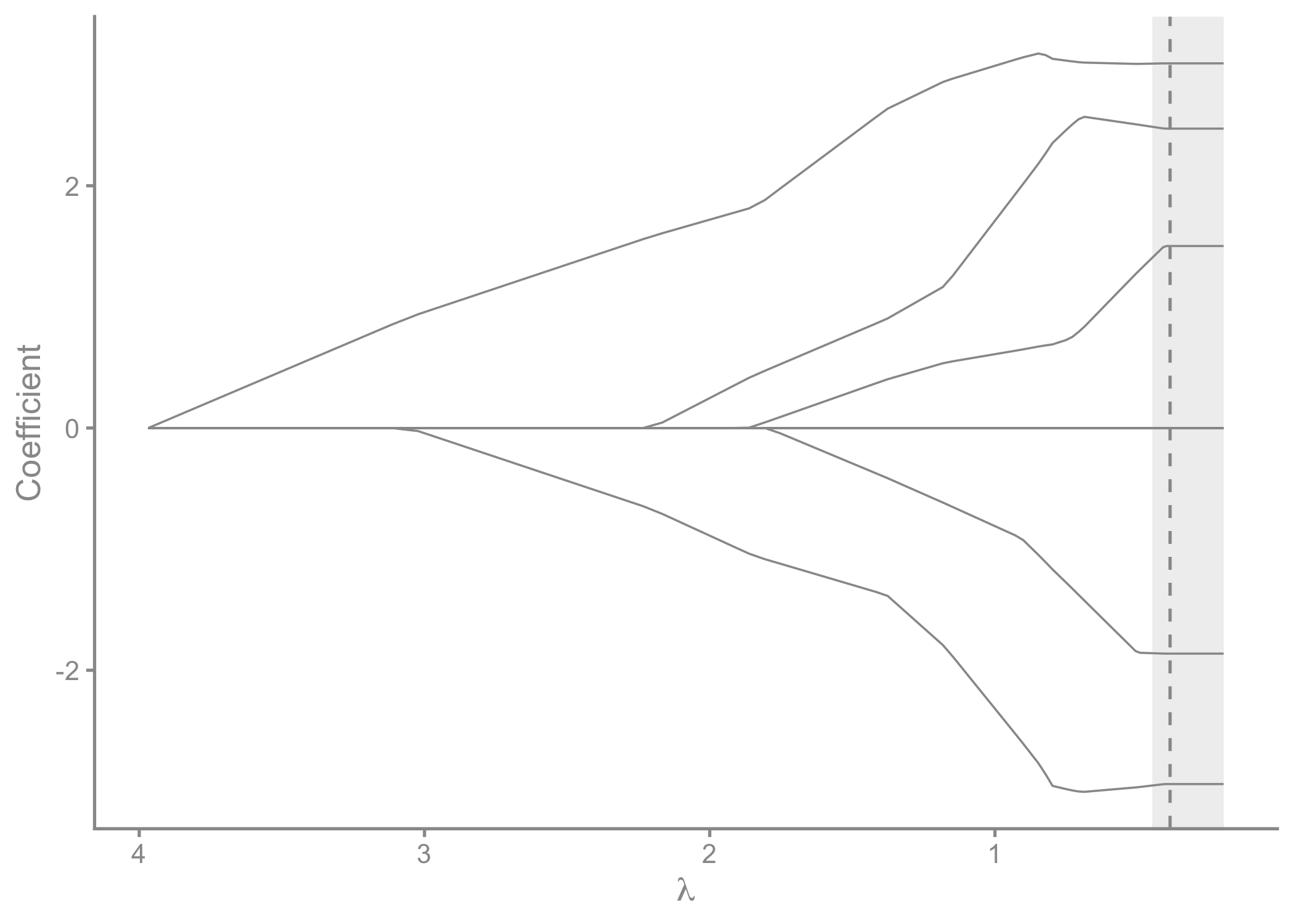
The coefficient path shows each estimate as a function of the penalty: for large \(\lambda\) every coefficient is zero, and as \(\lambda\) relaxes the true signals enter the model while the noise variables stay at zero. This is the SCAD estimator doing exactly what the derivation promised, selecting the sparse set of real effects and, thanks to the flat region of the penalty, estimating the strong ones without the bias the lasso would introduce.
Application: Classifying Leukemia from Gene Expression
Here, we use gene-expression data from 72 leukemia patients with measurements on 3,571 genes. Each patient belongs to one of two subtypes, acute myeloid leukemia (AML) or acute lymphoblastic leukemia (ALL). The goal is to classify leukemia subtype from gene expression. With more than three thousand genes and only 72 patients, this is a clear \(p \gg n\) setting. Because the outcome is binary, we use SCAD-penalized logistic regression, applying the SCAD penalty to the logistic loss rather than the least-squares loss.
library(spikeslab)
data(leukemia)

y_leuk <- leukemia[, 1]
X_leuk <- as.matrix(leukemia[, -1])

dim(X_leuk)
[1] 72 3571set.seed(1)
cv_leuk <- cv.ncvreg(X_leuk, y_leuk,
family = "binomial",
penalty = "SCAD",
gamma = 3.7)
coefs_leuk <- coef(cv_leuk)[-1]
selected_genes <- which(abs(coefs_leuk) > 1e-6)
length(selected_genes)[1] 11SCAD retains only a small set, the genes whose expression distinguishes the two leukemia subtypes, and zeroes out all the rest. We can list the selected genes and check how well the model separates the subtypes.
knitr::kable(
  data.frame(
  Gene        = selected_genes,
  Coefficient = round(coefs_leuk[selected_genes], 3)
),
digits = 3
)| Gene | Coefficient | |
|---|---|---|
| x.456 | 456 | -0.426 |
| x.626 | 626 | -0.275 |
| x.672 | 672 | -0.857 |
| x.956 | 956 | 0.365 |
| x.979 | 979 | 0.487 |
| x.1219 | 1219 | -0.068 |
| x.1652 | 1652 | 0.224 |
| x.1946 | 1946 | 0.160 |
| x.2481 | 2481 | 0.435 |
| x.3098 | 3098 | 0.172 |
| x.3441 | 3441 | -0.060 |
# Cross-validated error at the selected lambda
data.frame(
  Genes_selected = length(selected_genes),
  CV_error       = round(min(cv_leuk$cve), 4)
)
Genes_selected CV_error
1 11 0.3918library(ggplot2)
df <- data.frame(
gene = seq_along(coefs_leuk),
coef = coefs_leuk
)
ggplot(df, aes(x = gene, y = coef)) +
geom_segment(
aes(xend = gene, yend = 0),
color = "#0096c7"
) +
geom_hline(
yintercept = 0,
color = "grey60"
) +
labs(
x = "Gene index",
y = "SCAD coefficient"
)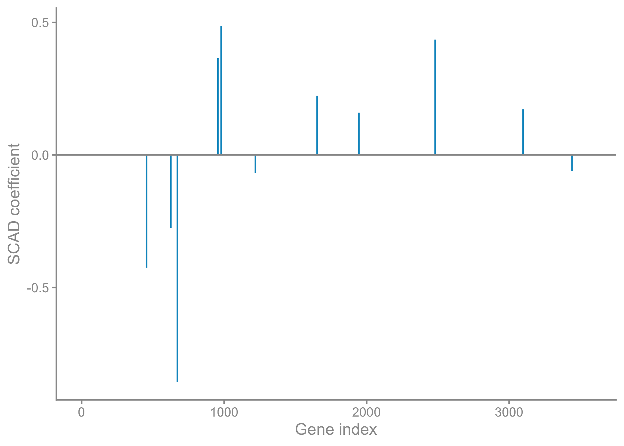
The coefficient plot shows the selected genes as spikes against a flat line of zeros. There are two important caveats. First, gene-expression variables are often correlated, so the specific genes selected can change with small changes in the data. The sparse signature is therefore better viewed as a starting point for validation than as a definitive set of genes. Second, with only 72 patients, the cross-validation results are also uncertain. The selected genes should therefore be treated as a hypothesis-generating shortlist rather than a final diagnostic panel. These limitations are common in high-dimensional genomic data and do not reflect a problem with SCAD itself.
References
Breheny, Patrick, and Jian Huang. 2011. “Coordinate Descent Algorithms for Nonconvex Penalized Regression, with Applications to Biological Feature Selection.” The Annals of Applied Statistics 5 (1): 232–53.
Fan, Jianqing, and Runze Li. 2001. “Variable Selection via Nonconcave Penalized Likelihood and Its Oracle Properties.” Journal of the American Statistical Association 96 (456): 1348–60.
Friedman, Jerome, Trevor Hastie, and Robert Tibshirani. 2010. “Regularization Paths for Generalized Linear Models via Coordinate Descent.” Journal of Statistical Software 33 (1): 1–22.
Tibshirani, Robert. 1996. “Regression Shrinkage and Selection via the Lasso.” Journal of the Royal Statistical Society: Series B (Methodological) 58 (1): 267–88.