library(truncnorm)
library(mice)
library(dplyr)
library(ggplot2)

mice.impute.trunc <- function(y, ry, x, wy = NULL,
                              trunc_type = c("below", "above", "interval"),
                              trunc_lower = NULL,
                              trunc_upper = NULL,
                              ...) {

  # values to impute
  if (is.null(wy)) {
    wy <- !ry
  }

  # observed data only
  xobs <- cbind(1, x[ry, , drop = FALSE])
  yobs <- y[ry]

  # fit regression model
  beta <- solve(
    t(xobs) %*% xobs,
    t(xobs) %*% yobs
  )

  # residual SD
  sigma <- sqrt(
    sum((yobs - xobs %*% beta)^2) /
      (length(yobs) - ncol(xobs))
  )

  # predictors for missing observations
  xmis <- cbind(1, x[wy, , drop = FALSE])

  # predicted means
  mu <- as.vector(xmis %*% beta)

  # choose truncation type
  trunc_type <- match.arg(trunc_type)

  if (trunc_type == "below") {
    if (is.null(trunc_upper)) {
      stop("For below truncation, specify trunc_upper")
    }
    imp <- rtruncnorm(
      n = sum(wy),
      a = -Inf,
      b = trunc_upper,
      mean = mu,
      sd = sigma
    )

  } else if (trunc_type == "above") {
    if (is.null(trunc_lower)) {
      stop("For above truncation, specify trunc_lower")
    }
    imp <- rtruncnorm(
      n = sum(wy),
      a = trunc_lower,
      b = Inf,
      mean = mu,
      sd = sigma
    )

  } else if (trunc_type == "interval") {
    if (is.null(trunc_lower) | is.null(trunc_upper)) {
      stop("For interval truncation, specify both trunc_lower and trunc_upper")
    }
    imp <- rtruncnorm(
      n = sum(wy),
      a = trunc_lower,
      b = trunc_upper,
      mean = mu,
      sd = sigma
    )
  }

  return(imp)
}Imputation with Bounds: A Truncated Method for mice
Missing Data
Statistics
R
mice
Intro
Multiple imputation is the standard remedy for missing data, and the mice package in R makes it easy to fill in gaps by drawing plausible values from a model fit to the observed data (Buuren and Groothuis-Oudshoorn 2011; Buuren 2018). Its default methods work well for variables that can, in principle, take any real value. But many variables in practice are bounded; for instance, a laboratory measurement cannot fall below its assay’s detection limit, a proportion must lie in [0, 1], an age cannot be negative, and a clinical score is confined to a fixed range. When such a variable is imputed with a method that assumes an unbounded distribution, nothing stops the imputation from producing values outside the permissible range.
These out-of-range imputations can distort the distribution the imputation is meant to preserve, bias downstream estimates, and cause models fitted to the completed data to behave poorly (Buuren 2018; Geraci and Farcomeni 2018). Naively clamping such values to the boundary afterward is worse, because it piles probability mass on the limits and misrepresents the shape of the distribution near the bounds.
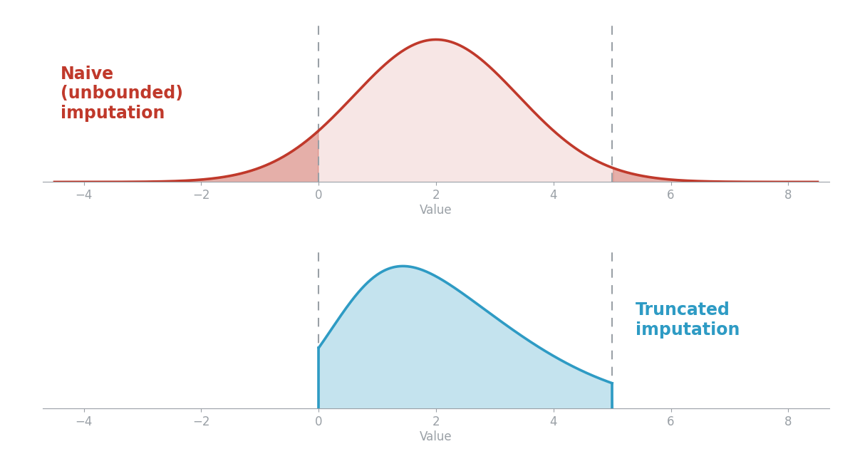
A cleaner solution is to impute from a distribution that respects the bounds from the outset. This can be done with different distributions depending on the variable and its assumed conditional distribution. For a variable modeled as approximately Gaussian conditional on covariates, the natural choice is a truncated normal distribution: the same regression model, but with draws restricted to the allowable interval (Geraci and Farcomeni 2018; Robert 1995). In this post, I implement a custom mice imputation method that does exactly this and show how to plug it into a standard mice workflow. I then use a simulated example to compare it against default imputation.
A Truncated-Normal Imputation Method
The mice function is extensible, and any function named mice.impute.<name> that follows the expected signature can be used by setting method = "<name>". The method fits an ordinary regression to the observed records, extracts the coefficient estimates and residual standard deviation, forms predicted means for the records requiring imputation, and then draws from a truncated normal distribution centered at those means. The truncation bounds are passed through the function and determine whether the distribution is truncated below, above, or to an interval.
The arguments y, ry, x, and wy are the standard mice interface: y is the variable being imputed, ry is the response indicator (TRUE where observed), x holds the predictors, and wy flags the records to impute (Buuren and Groothuis-Oudshoorn 2011). The bounds trunc_lower and trunc_upper are passed as extra arguments, and the trunc_type argument selects which side(s) to truncate. These are given a trunc_ prefix deliberately: mice uses an internal argument named type for its predictor matrix, so a custom argument also called type would collide and error. Draws come from rtruncnorm in the truncnorm package, which samples directly from a normal distribution restricted to [a, b] (Mersmann et al. 2018). The regression itself is fit only to the observed records, exactly as a standard imputation model would be.
One deliberately simple choice here is that the method conditions on point estimates of the regression coefficients rather than drawing them from their posterior. A fully proper multiple-imputation method would add that extra layer of uncertainty; the version above is a clear, transparent starting point, and I note below how it can be extended.
Example
Consider a cholesterol-like laboratory value bounded below by an assay detection limit and above by a physiological ceiling. Data are simulated such that the biomarker depends on age and a treatment indicator. A subset of biomarker values is then deleted completely at random, allowing the focus to remain on the bounding problem rather than on the missingness mechanism.
set.seed(42)
n <- 500

age       <- round(rnorm(n, 50, 10))
treatment <- rbinom(n, 1, 0.5)

# Biomarker that sits near its lower detection limit of 10.
# The bounds are [10, 90], but the data cluster close to the lower bound,
# which is exactly when respecting the limit matters.
biomarker <- 12 + 0.14 * age - 4 * treatment + rnorm(n, 0, 11)
biomarker <- pmin(pmax(biomarker, 10), 90)

dat <- data.frame(biomarker, age, treatment)

# Introduce missingness in the biomarker (MCAR for illustration)
miss_idx <- sample(1:n, size = 150)
dat$biomarker[miss_idx] <- NA

summary(dat$biomarker)
Min. 1st Qu. Median Mean 3rd Qu. Max. NAs
10.00 10.32 17.04 18.74 23.61 57.45 150 The observed biomarker clusters near its lower detection limit of 10, with a fraction of records sitting right at the floor. This is precisely the setting where the choice of imputation method matters: because the data hug the lower bound, an unbounded model will readily draw values below it. The question is whether an imputation method keeps the filled-in values inside the plausible window.
Because the function is named mice.impute.trunc, it can be requested by setting method = "trunc" for the biomarker while leaving the fully observed predictors unchanged. The truncation bounds are supplied through the ... mechanism that mice forwards to the imputation method.
# only the biomarker needs imputation
meth <- make.method(dat)
meth["biomarker"] <- "trunc"

# Impute with interval truncation on [10, 90]
imp_trunc <- mice(
  dat,
  method = meth,
  m = 5,
  trunc_type = "interval",
  trunc_lower = 10,
  trunc_upper = 90,
  printFlag = FALSE,
  seed = 1
)
For comparison, a default imputation is performed using Bayesian linear regression (norm), which does not impose any restrictions on the range of the imputed values.
meth_naive <- make.method(dat)
meth_naive["biomarker"] <- "norm"

imp_naive <- mice(
  dat,
  method = meth_naive,
  m = 5,
  printFlag = FALSE,
  seed = 1
)
The clearest diagnostic is the range of the imputed values. Imputed biomarker values are extracted from the first completed dataset under each approach, and the number of values falling outside the plausible range is then recorded.
trunc_vals <- complete(imp_trunc, 1)$biomarker[is.na(dat$biomarker)]
naive_vals <- complete(imp_naive, 1)$biomarker[is.na(dat$biomarker)]

data.frame(
  Method = c("Truncated", "Naive (norm)"),
  Min    = c(min(trunc_vals), min(naive_vals)),
  Max    = c(max(trunc_vals), max(naive_vals)),
  `Out of [10, 90]` = c(
    sum(trunc_vals < 10 | trunc_vals > 90),
    sum(naive_vals < 10 | naive_vals > 90)
  ),
  check.names = FALSE
)
Method Min Max Out of [10, 90]
1 Truncated 10.068074 40.27381 0
2 Naive (norm) -9.546317 45.34098 22The truncated method keeps every imputed value inside [10, 90], while the naive normal imputation produces a substantial number of out-of-range values, including negative biomarker measurements, which are impossible.
plot_df <- bind_rows(
  data.frame(value = dat$biomarker[!is.na(dat$biomarker)], source = "Observed"),
  data.frame(value = trunc_vals, source = "Imputed (truncated)"),
  data.frame(value = naive_vals, source = "Imputed (naive)")
)

ggplot(plot_df, aes(x = value, fill = source)) +
  geom_density(alpha = 0.45) +
  labs(x = "Biomarker value", y = "Density", fill = NULL)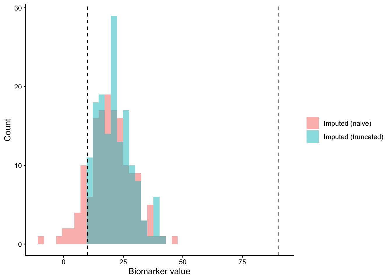
To isolate the behavior of the two methods, it helps to drop the observed data and plot only the imputed values against the bounds. The observed values are in-bounds by construction and are not what is failing here, so removing them puts the contrast we care about, naive versus truncated.
imp_df <- bind_rows(
  data.frame(value = trunc_vals, source = "Imputed (truncated)"),
  data.frame(value = naive_vals, source = "Imputed (naive)")
)

ggplot(imp_df, aes(x = value, fill = source)) +
  geom_histogram(alpha = 0.5, position = "identity", bins = 40) +
  geom_vline(xintercept = c(10, 90), linetype = "dashed") +
labs(x = "Biomarker value", y = "Count", fill = NULL) 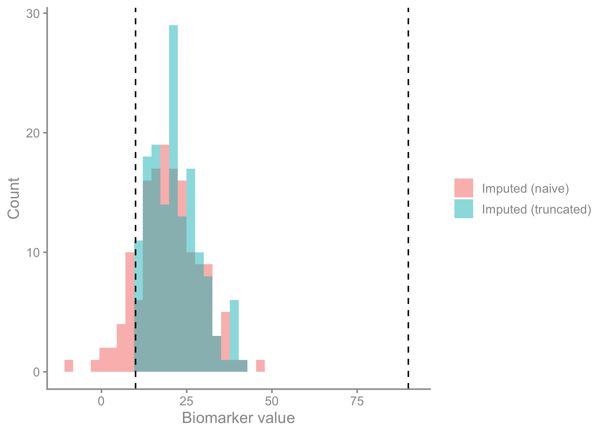
The naive density extends left across the lower bound and into negative territory (impossible values for a biomarker) while the truncated density terminates exactly at the boundary. This is the same information the out-of-bounds count conveyed numerically, now shown as the shape of the two imputation distributions.
Note that the method above is intentionally minimal, and two extensions make it more fully “proper” in Rubin’s sense (Buuren 2018). First, rather than conditioning on point estimates of the regression coefficients, one can draw them from their posterior (sampling \(\sigma\) from its scaled inverse-chi-squared distribution and \(\beta\) from its conditional normal) so that the imputations reflect estimation uncertainty in the model, not just residual variability. Second, the bounds themselves can be made variable-specific or even record-specific (for instance, a detection limit that differs across assay batches) by passing vectors of lower and upper, since rtruncnorm accepts vectorized bounds. Both extensions slot cleanly into the same structure.
Bounded variables are everywhere in health data, and imputing them with unbounded models can produce impossible values that distort the analysis. When your data have meaningful limits, it is worth making your imputations respect them.
References
Buuren, Stef van. 2018. Flexible Imputation of Missing Data. 2nd ed. Chapman; Hall/CRC.
Buuren, Stef van, and Karin Groothuis-Oudshoorn. 2011. “Mice: Multivariate Imputation by Chained Equations in r.” Journal of Statistical Software 45 (3): 1–67.
Geraci, Marco, and Alessio Farcomeni. 2018. “Mid-Quantile Regression for Discrete Responses.” Statistical Methods in Medical Research.
Mersmann, Olaf, Heike Trautmann, Detlef Steuer, and Bjoern Bornkamp. 2018. Truncnorm: Truncated Normal Distribution. https://CRAN.R-project.org/package=truncnorm.
Robert, Christian P. 1995. “Simulation of Truncated Normal Variables.” Statistics and Computing 5 (2): 121–25.