How do you answer a question you never got to run the experiment for? Suppose you run a six-month exercise program (or intervention) and want to know whether it lowers systolic blood pressure (SBP). The tempting move is to compare the average SBP of people who enrolled against people who didn’t and call the difference the program’s effect.
That comparison does answer a question. It tells you whether people who enrolled in the program had different average SBP than those who did not. But it does not tell you whether the difference was caused by the program. The two groups may differ in many other ways. If clinicians were more likely to refer patients with higher blood pressure or other risk factors to the program, for example, the people who enrolled may have started out sicker. A simple comparison would then mix the effect of the program with the differences that existed between the groups before the program began.
The question you actually want to answer is counterfactual. What would the average SBP have been if everyone in the population had been enrolled in the program, compared with what it would have been if no one had enrolled?
The problem is that you can never see what would have happened to the same person under both choices. If someone enrolls in the program, you observe what their SBP is after the program, but you do not know what their SBP would have been if they had not enrolled. If someone does not enroll, you observe their SBP without the program, but you do not know what their SBP would have been if they had enrolled. For each person, one of these two outcomes is always unobserved.
G computation provides a way to reason about these missing outcomes. You fit a model that describes how outcomes depend on treatment and the characteristics of each person. You then use that model to predict what each person’s outcome would have been if they had enrolled and what it would have been if they had not. This allows you to construct the two hypothetical worlds for everyone in the population and compare their average outcomes (see Robins (1986) for the original formulation and (2011) and Hernán & Robins (2020) for a detailed presentation).
The estimand you are chasing here is the average treatment effect (ATE): \[
\small{\text{ATE} \;=\; \text{E}\big[\,\text{E}[Y \mid A = 1, \mathbf{W}]\; -\; \text{E}[Y \mid A = 0, \mathbf{W}]\,\big]}
\] Here, \(Y\) is the outcome, \(A\) is the binary treatment (\(1\) = treated, \(0\) = control), and \(\mathbf{W} = (W_1, W_2, \dots, W_p)\) represents the baseline characteristics measured before treatment. The inner expectations are model based predictions for a person with covariates \(\mathbf{W}\). One prediction asks what their expected outcome would be under treatment, and the other asks what it would be under no treatment. The outer expectation then averages these individual level contrasts over the covariate distribution of the population you care about.
Note
The ATE is not the only causal effect you can estimate using g-computation. The same approach can be adapted to target the average treatment effect among the treated (ATT) or the average treatment effect among the untreated (ATU). The key difference is the population over which you average the predicted treatment contrasts. For the ATE, you average over everyone in the population. For the ATT, you average over the people who actually received treatment. For the ATU, you average over the people who did not receive treatment. The model and the counterfactual predictions can remain the same.
These three estimands are related. Because everyone in the population either enrolled or did not enroll, the ATE can be written as a weighted average of the ATT and ATU:
\[
\boxed{
\small{\text{ATE}
=
\pi_p*\text{ATT}
+
(1-\pi_p)*\text{ATU}
}}
\] where \(\pi_p\) is the proportion of the population who enrolled in the program.
We will focus on estimating the ATE throughout the main example, and at the end we will return to the same fitted model and show how to obtain the ATT and ATU.
Now, let’s consider a simulation where we know the answer. The nice thing about simulated data is that we can peek at the truth and grade ourselves. Here, being older, heavier, and a smoker all raise SBP and also raise the chance of being referred to the program.
n <-3000dat <-tibble(age =round(rnorm(n, mean =54, sd =11)),bmi =round(rnorm(n, mean =28, sd =4.5), 1),smoker =rbinom(n, 1, 0.22)) %>%mutate(# sicker patients are more likely to be referred to the programp_enroll =plogis(-9.0+0.09* age +0.16* bmi +0.90* smoker),program =rbinom(n, 1, p_enroll),# true structural model for SBP; program effect is -6 mmHgsbp =118+0.75* (age -54) +1.40* (bmi -28) +8.0* smoker +-6.0* program +rnorm(n, 0, 8) ) %>%select(age, bmi, smoker, program, sbp)head(dat)
age
bmi
smoker
program
sbp
52
31.8
0
1
120.7437
54
34.3
0
1
109.0062
53
27.4
0
0
126.8229
60
26.4
0
1
109.9852
55
25.0
0
1
123.2858
68
33.8
0
0
136.4456
By construction, the true ATE is −6 mmHg. Every person’s SBP would be 6 points lower under the program than without it. Before trying to estimate that effect, let’s look at the baseline characteristics of people who enrolled and those who did not.
Enrollees are roughly 8 years older, 2.3 BMI units heavier, and about 11 percentage points more likely to smoke. So, a simple comparison of mean SBP between the two groups may not recover the causal effect of the program because the groups differ systematically in characteristics that may affect SBP.
To see the consequence of ignoring these differences, let’s calculate the naive comparison of mean SBP between enrollees and non-enrollees without adjusting for \(\mathbf{W} = (\)age, bmi, smoker\()\).
The unadjusted difference is about +4.1 mmHg, which has the wrong sign. The program actually lowers SBP by 6 mmHg, yet the naive comparison suggests that it raises SBP by about 4 mmHg. This happens because the people who enroll are older, have higher BMI, and are more likely to smoke. These characteristics are also associated with higher SBP, so enrollees would tend to have higher SBP even without the program. The program lowers their SBP by 6 mmHg, but not enough to overcome the baseline differences between the groups. The observed difference is therefore positive.
The naive comparison mixes the effect of the program with the preexisting differences between the groups. In this example, those differences are large enough to completely reverse the direction of the estimated effect.
Now that we have seen how the naive comparison can be misleading, let’s adjust for age, BMI, and smoking to estimate the program effect using g-computation.
Step 1: Fit the outcome model
The first step is to fit an outcome model by regressing the outcome on treatment and the covariates. This model is a prediction machine. The goal here is not to interpret its coefficients individually.
Now comes the counterfactual part. Create two copies of the dataset. In the first copy, set everyone’s treatment to 1, whether or not they actually enrolled. In the second, set everyone’s treatment to 0, whether or not they actually stayed out of the program. The important point is that you change only the treatment variable. You leave age, BMI, and smoking exactly as they were because you are asking what would happen if treatment were changed while keeping the population itself the same.
dat_all_treated <- dat %>%mutate(program =1)dat_all_control <- dat %>%mutate(program =0)
Then push both copies through the fitted model:
y1_hat <-predict(outcome_fit, newdata = dat_all_treated, type ="response")y0_hat <-predict(outcome_fit, newdata = dat_all_control, type ="response")
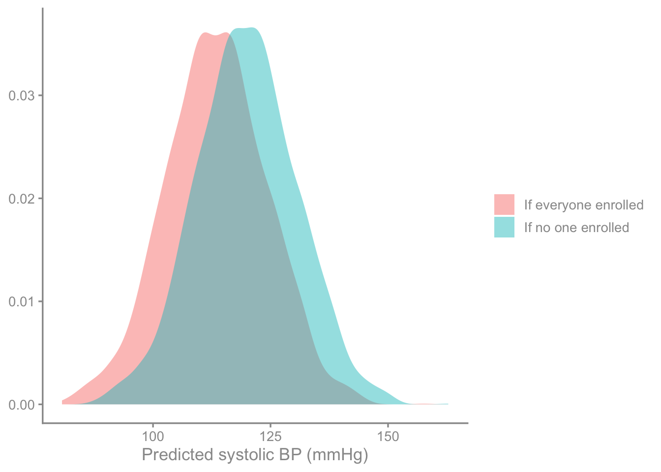
y1_hat is a vector of \(\hat{E}[Y \mid A = 1, \mathbf{W}]\), one entry per person; y0_hat is the same for \(A = 0\). For any given person, one of these is a prediction of something that actually happened and the other is a prediction of a world that never occurred, and the model treats them identically.
For each person, one prediction corresponds to the treatment they actually received and the other corresponds to an outcome that was never observed. The fitted model gives you a way to predict that missing outcome.
tibble(value =c(y1_hat, y0_hat),world =rep(c("If everyone enrolled", "If no one enrolled"), each = n)) %>%ggplot(aes(value, fill = world)) +geom_density(alpha =0.45, colour =NA) +labs(x ="Predicted systolic BP (mmHg)", y =NULL, fill =NULL)
Step 3: Average the difference
Now calculate the difference between the two predictions for each person and average those differences across the population.
\[
\widehat{\text{ATE}} \;=\; \frac{1}{n}\sum_{i=1}^{n}\Big(\hat{E}[Y \mid A = 1, \mathbf{W}_i] - \hat{E}[Y \mid A = 0, \mathbf{W}_i]\Big)
\]
Close to −6.
Now, we can use the nonparametric bootstrap to obtain the confidence interval for the estimate. Resample people with replacement and repeat the entire g-computation procedure within each bootstrap sample. This means fitting the model again and generating the counterfactual predictions again.
gcomp_once <-function(data) { fit <-glm(sbp ~ program*(age + bmi + smoker), data = data, family =gaussian())mean(predict(fit, newdata =mutate(data, program =1), type ="response") -predict(fit, newdata =mutate(data, program =0), type ="response") )}boot_ate <-map_dbl(1:1000, \(i) { idx <-sample(nrow(dat), replace =TRUE)gcomp_once(dat[idx, ])})tibble(estimate = ate_gcomp,se =sd(boot_ate),conf.low =quantile(boot_ate, 0.025),conf.high =quantile(boot_ate, 0.975)) %>%mutate(across(everything(), \(x) round(x, 2)))
estimate
se
conf.low
conf.high
-6.39
0.34
-7.06
-5.72
Note
Nothing fundamental changes when \(Y\) is binary. You still fit an outcome model, predict the outcome under both treatment levels for every person, and average the resulting contrasts. The main difference is that you can choose which marginal effect measure you want to report.
Once the mechanics are clear, you can use a package to handle the prediction and averaging for you. marginaleffects implements this and can also provide uncertainty estimates.
 Estimate Std. Error   z Pr(>|z|)     S 2.5 % 97.5 %
    -6.39      0.337 -19   <0.001 263.7 -7.05  -5.73

Term: program
Type: response
Comparison: 1 - 0
The ATE is only one of the causal effects you can estimate with this approach. Recall that the ATE averages the individual treatment contrasts over everyone in the population. If your question is instead about the effect among people who actually enrolled, you want the ATT. If your question is about the effect among people who did not enroll, you want the ATU.
The counterfactual predictions are the same in all three cases. What changes is the population over which those predictions are averaged. marginaleffects lets you make that distinction directly by specifying the subset of the population over which the comparison should be averaged.
For the ATT, average the treatment contrast among those who actually enrolled:
 Estimate Std. Error     z Pr(>|z|)     S 2.5 % 97.5 %
    -6.44      0.352 -18.3   <0.001 246.1 -7.13  -5.75

Term: program
Type: response
Comparison: 1 - 0
References
Hernán, Miguel A., and James M. Robins. 2020. Causal Inference: What If. Chapman & Hall/CRC.
Robins, James. 1986. “A New Approach to Causal Inference in Mortality Studies with a Sustained Exposure Period—Application to Control of the Healthy Worker Survivor Effect.”Mathematical Modelling 7 (9–12): 1393–512. https://doi.org/10.1016/0270-0255(86)90088-6.
Snowden, Jonathan M, Sherri Rose, and Kathleen M Mortimer. 2011. “Implementation of g-Computation on a Simulated Data Set: Demonstration of a Causal Inference Technique.”American Journal of Epidemiology 173 (7): 731–38. https://doi.org/10.1093/aje/kwq472.