Propensity Score Matching & ATT Estimation using G-Computation
Motivation
Causal inference is essential in medical research for establishing cause-and-effect relationships between variables. While randomized controlled trials (RCTs) are the gold standard for evaluating interventions, they are not always feasible or ethical. In such cases, observational studies become crucial, albeit with challenges in making causal inferences due to the absence of randomization. This lack of randomization makes it difficult to isolate treatment effects from other influential factors, which can complicate attributing differences in outcomes to the treatment itself. Furthermore, self-selection bias, where patients choose treatments based on personal reasons, may introduce systematic differences between treated and untreated groups. It becomes necessary to account for these variations in observed characteristics when analyzing observational studies (Cochran 1965; Austin 2011).
Propensity score matching (PSM) has emerged as a valuable tool for addressing the challenges of estimating treatment effects in observational studies. This method involves estimating the likelihood of receiving a treatment, denoted as \(\tau\), based on observed covariates \(X_i\), which is mathematically represented as \(e(X) = \text{P}(\tau=1|X_1, \dots, X_n)\) (Rosenbaum and Rubin 1983, 1985; D’Agostino Jr 1998; Austin 2008). The entire process of PSM includes estimating propensity scores, matching treated and control subjects based on these scores, conducting balance diagnostics to ensure comparable groups, and finally, estimating the treatment effect. By achieving balance between the treated and control groups on these covariates, PSM aims to minimize confounding and improve the accuracy of treatment effect estimation.
One of the key measures (or effect estimate) of interest after matching is the Average Treatment Effect on the Treated (ATT). The ATT represents the average effect of the treatment on those subjects who actually received it. It does so by comparing the actual outcomes of treated subjects with their counterfactual outcomes—what would have happened if they had not received the treatment (Wang, Nianogo, and Arah 2017; Greifer and Stuart 2023). This measure is particularly relevant in observational studies, where understanding the intervention’s impact on the population that chose to undergo treatment is crucial (refer to Greifer and Stuart (2023) for detailed guidelines on choosing the causal estimand). In this context, the ATT is essential for evaluating the effectiveness of interventions in real-world settings, as it provides insights into the benefits received by those who opted for the treatment (Imbens 2004).
To estimate the ATT, g-computation has emerged as a powerful technique that has gained popularity in recent times (Robins 1986; Snowden, Rose, and Mortimer 2011; Chatton et al. 2020). This method involves specifying a model for the outcome and then using this model to predict potential outcomes under different treatment scenarios. By comparing these predicted outcomes, researchers can estimate the causal effect of the treatment on the treated population. G-computation is flexible and can handle complex covariate structures and interactions, accommodate time-varying treatments and covariates, and provide estimates that are less biased in the presence of model misspecification compared to other methods. However, it requires careful model specification and validation to ensure accurate and reliable estimates.
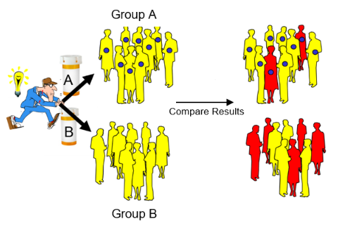
In this blog post, we will demonstrate how to implement PSM and estimate ATT using g-computation. We will start by generating synthetic data, calculating propensity scores, and performing matching. Finally, we will estimate the ATT with confidence intervals. By the end of this post, you will have a solid understanding of these methods and their practical applications in effect estimation.
Generating Synthetic Data
We begin by generating synthetic data, including variables such as age, weight, pre-existing conditions, smoking status, and cholesterol level. Treatment assignment will be random, with outcomes affected by these variables and the treatment itself.
# Set seed for reproducibility
set.seed(42)

# Generate synthetic data
n <- 5000

# Treatment assignment
treatment <- rbinom(n, 1, 0.5)

# Baseline Characteristics
age <- round(rnorm(n, 50, 10))
weight <- round(rnorm(n, 70, 15), 2)
conditions <- rbinom(n, 1, 0.3)
smoking <- rbinom(n, 1, 0.2 + 0.2 * treatment) # more smokers in treatment group
exercise <- rbinom(n, 1, 0.5 - 0.2 * treatment) # less exercise in treatment group
cholesterol <- round(rnorm(n, 200 + 20 * treatment, 30), 2) # higher cholesterol in treatment group
gender <- rbinom(n, 1, 0.5)

# Outcome (binary)
# True treatment effect is reduction in the probability of the binary outcome
baseline_logit <- -5 + 0.05 * age + 0.03 * weight + 0.5 * conditions + 0.2 * smoking - 0.3 * exercise + 0.01 * cholesterol + 0.15 * gender
treatment_effect <- -1 # log-odds reduction due to treatment
logit <- baseline_logit + treatment * treatment_effect
prob <- exp(logit) / (1 + exp(logit))
outcome <- rbinom(n, 1, prob)

# Create data frame
data <- data.frame(
  age = age,
  weight = weight,
  conditions = conditions,
  smoking = smoking,
  exercise = exercise,
  cholesterol = cholesterol,
  gender = gender,
  treatment = treatment,
  outcome = outcome
)

head(data)| age | weight | conditions | smoking | exercise | cholesterol | gender | treatment | outcome |
|---|---|---|---|---|---|---|---|---|
| 56 | 74.40 | 0 | 0 | 1 | 202.17 | 0 | 1 | 0 |
| 50 | 63.94 | 0 | 0 | 1 | 213.52 | 0 | 1 | 0 |
| 49 | 37.30 | 0 | 0 | 1 | 202.51 | 0 | 0 | 0 |
| 54 | 72.96 | 0 | 0 | 0 | 236.17 | 0 | 1 | 1 |
| 56 | 98.84 | 1 | 0 | 0 | 242.95 | 0 | 1 | 1 |
| 50 | 56.08 | 0 | 0 | 1 | 217.64 | 0 | 1 | 1 |
Evaluating Covariate Balance in the Original Data
Next, we examine the difference in baseline characteristics between the treated and control groups using standardized mean differences (SMD). An absolute SMD greater than 0.1 indicates significant imbalance (Normand et al. 2001; Daniel E. Ho et al. 2007; Stuart, Lee, and Leacy 2013).
| Summary of Original Data | |||||
|---|---|---|---|---|---|
| Comparison of Treated and Control Groups in the Original Data | |||||
| Variable | Means Treated | Means Control | SMD | eCDF Mean | eCDF Max |
| distance | 0.589 | 0.419 | 0.898 | 0.238 | 0.354 |
| age | 50.067 | 49.709 | 0.036 | 0.006 | 0.031 |
| weight | 70.077 | 69.625 | 0.030 | 0.009 | 0.026 |
| conditions | 0.293 | 0.308 | −0.034 | 0.015 | 0.015 |
| smoking | 0.408 | 0.199 | 0.425 | 0.209 | 0.209 |
| exercise | 0.300 | 0.513 | −0.465 | 0.213 | 0.213 |
| cholesterol | 219.957 | 200.842 | 0.627 | 0.166 | 0.252 |
| gender | 0.504 | 0.508 | −0.007 | 0.003 | 0.003 |
The table above shows that there are systematic differences in the distribution of smoking status, cholesterol level and those who exercise between the treated and control subjects. These differences underline the necessity for propensity score matching to control for confounding variables and ensure a balanced comparison between the groups.
Matching
After assessing covariate balance in the original data, we proceed with PSM using optimal full matching (see Optimal Full Matching and Matching Methods for detailed description) from the MatchIt package (Daniel E. Ho et al. 2011).
covars <- setdiff(colnames(data), c("treatment", "outcome"))
formula <- as.formula(paste("treatment ~", paste(covars, collapse = " + ")))

matchit_ <- matchit(formula, data = data, method = "full")
matched_data <- match.data(matchit_)
Balance Diagnostics
To ensure the effectiveness of the matching, we need to conduct balance diagnostics to examine the covariate distributions post-matching. To visually represent covariate balance, we use a love.plot, showing SMDs before and after matching.
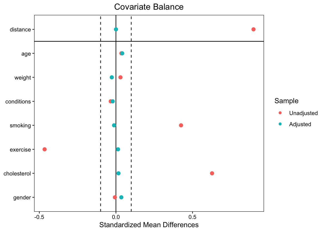
The plot shows that balance was improved on all variables after matching, bringing all SMDs below the threshold of 0.1.
Estimating ATT with G-Computation
Once the covariate balance is assessed and confirmed, the next step is to estimate the effect of the treatement on the outcome. This estimation provides insights into the differential impact of the treatment on the outcome. In the ATT estimation, we will use the g-computation process. We begin by extracting the matched dataset from the PSM procedure and fitting a generalized linear model (GLM) to the matched dataset. Next, we create a subset of the matched data that includes only the treated subjects. The GLM model is then used to predict the outcome probabilities for the treated subjects under both treated and control scenarios. The expected potential outcomes is then computed as weighted means of the predicted probabilities, yielding estimates of the average outcome under treatment (\(p_1\)) and control (\(p_0\)) conditions for the treated group.
Here, the ATT can be measured by calculating the risk ratio (RR), the absolute risk reduction (ARR), and the number needed to treat (NNT). RR is the ratio of the expected potential outcomes under treatment to those under control for the treated units, which measures the relative increase in the likelihood of the outcome due to the treatment among the treated individuals. Specifically, RR is computed as \(p_1/p_0\). An RR greater than 1 indicates an increased risk in the treated group, while an RR less than 1 indicates a decreased risk. On the other hand, the ARR quantifies the difference in the event rates of the outcome between the treated and control groups. Precisely, ARR is estimated as \(p_0-p_1\), providing a straightforward measure of the risk reduction attributable to the treatment. The inverse of the ARR is the NNT, and it indicates the average number of individuals who need to be treated to prevent one additional bad outcome.
To facilitate this process, we have created a function, att_boot, which allows users to specify the specific measure of interest — RR, ARR, or NNT. The function uses bootstrapping to estimate these measures, providing flexibility and robustness in the analysis. Users can easily compute the desired metric based on their research needs, making the process of ATT estimation both comprehensive and user-friendly.
To ensure the robustness of the estimates and to find the confidence intervals, we will conduct 500 bootstrap replications using the bias-corrected and accelerated (BCa) bootstrap method with the bcaboot package (Efron and Narasimhan 2021, 2020; DiCiccio and Efron 1996; Efron 1987). This is done in the function estimate_bca, which also uses the att_boot function. Each replication encompasses the entire process of GLM fitting and g-computation. The BCa method is being used to adjust for bias and skewness in the bootstrap distribution, providing more accurate confidence intervals than standard percentile intervals.
att_boot <- function(data, index, covars, measure = "RR") {
  formula <- as.formula(paste("outcome", "~ treatment * (", paste(covars, collapse = " + "), ")"))

  # Bootstrap sample
  data_boot <- data[index, ]

  # Fit the model
  fit <- glm(formula, data = data_boot, weights = data_boot$weights, family = quasibinomial())

  # Subset data for those with treatment == 1
  boot_data <- subset(data_boot, treatment == 1)

  # Predicted probabilities for the scenario treatment = 0
  prob0 <- predict(fit, type = "response", newdata = transform(boot_data, treatment = 0))
  prob_w0 <- weighted.mean(prob0, boot_data$weights)

  # Predicted probabilities for the scenario treatment = 1
  prob1 <- predict(fit, type = "response", newdata = transform(boot_data, treatment = 1))
  prob_w1 <- weighted.mean(prob1, boot_data$weights)

  # Calculate measures based on user input: RR, ARR, NNT
  # RR: Relative Risk
  # ARR: Absolute Risk Reduction
  # NNT: Number Needed to Treat

  if (measure == "RR") {
    result <- prob_w1 / prob_w0
  } else if (measure == "ARR") {
    result <- prob_w0 - prob_w1
  } else if (measure == "NNT") {
    ARR <- prob_w0 - prob_w1
    result <- ifelse(ARR != 0, 1 / ARR, NA) # Avoid division by zero
  } else {
    stop("Invalid measure specified. Choose 'RR', 'ARR', or 'NNT'.")
  }

  return(result)
}

estimate_bca <- function(data, covars, measure = "RR", B = 500, m = 40) {
  bca <- bcajack2(data, function(data, index) att_boot(data, index, covars, measure), B = B, m = m, verbose = FALSE)
  return(bca)
}
To test the functionalities of our ATT estimation process, we can use the following code snippets. These examples demonstrate how to apply the function to a matched dataset and obtain specific measures of interest, such as the RR, ARR and the NNT.
First, to estimate the Absolute Risk Reduction (ARR), we can use the following code:
bca_results <- estimate_bca(matched_data, covars, measure = "ARR")
print(bca_results)
$call
bcajack2(x = data, B = B, func = function(data, index) att_boot(data,
index, covars, measure), m = m, verbose = FALSE)
$lims
bca jacksd std pct
0.025 0.08910425 0.0044143569 0.09160756 0.020
0.05 0.09534177 0.0021192595 0.09799534 0.044
0.1 0.10349628 0.0031786440 0.10536006 0.094
0.16 0.11135144 0.0016761561 0.11117990 0.156
0.5 0.13123244 0.0009035576 0.13133915 0.502
0.84 0.15271882 0.0025032727 0.15149839 0.836
0.9 0.15692126 0.0023775723 0.15731824 0.894
0.95 0.16121304 0.0034664549 0.16468295 0.944
0.975 0.16884683 0.0064537618 0.17107074 0.970
$stats
theta sdboot z0 a sdjack
est 0.1313391 0.0202715921 0.005013278 -0.0215371727 0.0212790246
jsd 0.0000000 0.0007148427 0.053902750 0.0008376149 0.0003883903
$B.mean
[1] 500.0000000 0.1313202
$ustats
ustat sdu
0.13135813 0.02267225
attr(,"class")
[1] "bcaboot"The results for the Absolute Risk Reduction (ARR) estimation using the BCa bootstrap are summarized below:
Point Estimate (θ̂): The point estimate of the ARR is approximately 0.1313. This means that, on average, the treatment reduces the risk of the outcome by about 13.13% in the treated group compared to the control group.
Bootstrap Standard Deviation (sdboot): The bootstrap estimate of the standard deviation is 0.0203, which gives an indication of the variability in the ARR estimate across bootstrap samples.
-
Bias-Corrected and Accelerated (BCa) Confidence Intervals:
- The 0.025 quantile indicates a lower bound of approximately 0.0891.
- The 0.975 quantile provides an upper bound of around 0.1688.
These values represent the limits of the 95% BCa confidence interval for the ARR, suggesting that the true ARR lies between these values with 95% confidence.
Jackknife Standard Error (sdjack): The jackknife estimate of the standard error is 0.0213. This is another measure of the variability of the ARR estimate.
The results indicate that the treatment is associated with a meaningful reduction in the risk of the outcome. The confidence intervals suggest that this effect is statistically significant, as the intervals do not cross zero. This reinforces the conclusion that the treatment likely has a beneficial effect on reducing the risk in the treated population.
Next, to estimate the Number Needed to Treat (NNT), we can modify the measure parameter accordingly:
bca_results <- estimate_bca(matched_data, covars, measure = "NNT")
print(bca_results)
$call
bcajack2(x = data, B = B, func = function(data, index) att_boot(data,
index, covars, measure), m = m, verbose = FALSE)
$lims
bca jacksd std pct
0.025 6.133419 0.05061201 5.368541 0.028
0.05 6.345433 0.07024118 5.729532 0.054
0.1 6.569150 0.11319165 6.145730 0.104
0.16 6.822728 0.04986551 6.474625 0.164
0.5 7.608978 0.05682219 7.613876 0.500
0.84 8.779548 0.14022643 8.753127 0.844
0.9 9.250969 0.25804604 9.082022 0.904
0.95 10.202235 0.26999826 9.498221 0.954
0.975 10.982804 0.22635988 9.859211 0.978
$stats
theta sdboot z0 a sdjack
est 7.613876 1.14560020 0.00000000 0.016993100 1.13714372
jsd 0.000000 0.04104128 0.05411406 0.001598588 0.05131752
$B.mean
[1] 500.000000 7.828356
$ustats
ustat sdu
7.399396 1.154271
attr(,"class")
[1] "bcaboot"The estimate of the NNT is approximately 8 (95% CI 6, 11). This indicates that, on average, about 8 individuals need to be treated to prevent one additional adverse outcome. This measure is particularly useful for interpreting the practical implications of the treatment effect in clinical or policy settings.
These examples illustrate how to use our functions to extract different measures of treatment effect, making the analysis flexible and tailored to specific research questions.
Conclusion
This post provided an in-depth guide to implementing Propensity Score Matching (PSM) and estimating the Average Treatment Effect on the Treated (ATT) using g-computation. Through this approach, we can effectively address confounding in observational studies, ensuring more accurate causal inferences. The combination of PSM and g-computation, along with robust diagnostics like the BCa bootstrap, offers a powerful toolkit for making credible causal inferences from real-world data. Thank you for reading, and I welcome your feedback. Feel free to share your thoughts and experiences with these methods!