Cluster-randomized trials (CRTs) randomize intact groups (like clinics, schools, villages) rather than individuals, and are widely used when interventions are delivered at the group level or when individual randomization may lead to contamination between study arms (Murray 1998; Hayes and Moulton 2017). CRTs often involve a relatively small number of randomized units, with some trials allocating as few as ten or twenty clusters across two arms. When the number of clusters is small, simple randomization can, by chance alone, produce substantial differences between study arms in important cluster-level covariates (Ivers et al. 2012; Moulton 2004). This imbalance can confound estimated intervention effects, and analyses that adjust for many cluster-level covariates quickly exhaust the limited degrees of freedom available in a small-cluster trial. Unlike individually randomized studies, where the law of large numbers tends to balance covariates across arms, CRTs offer no such guarantee, precisely because the unit of randomization is scarce (Li et al. 2016).
Covariate-constrained randomization (CCR) addresses this problem. Rather than accepting whatever allocation simple randomization produces, CCR restricts the randomization to the subset of allocations that achieve acceptable balance on prespecified covariates (Raab and Butcher 2001; Moulton 2004). The procedure is to:
Enumerate the space of possible allocations.
Score each one with a balance criterion.
Retain only those allocations meeting the criterion.
Randomly select the final allocation from this constrained set.
This preserves randomization and help exclude highly imbalanced allocations that can arise by chance in small trials (Li et al. 2016). A key design question in CCR is how tightly to constrain. Restrict too little and imbalance remains; restrict too aggressively and the constrained set becomes small, which can compromise the validity of randomization-based inference and inflate the correlation between allocation and covariates (Bailey 1987; Li et al. 2017).
This post implements CCR for a two-arm cluster trial. Cluster-level covariates are generated, a balance metric is defined, candidate allocations are enumerated, the constrained randomization space is constructed, and the balance achieved under constrained and simple randomization is compared. Table 1-style covariate is produced to assess balance summary after randomization to confirm the arms are comparable.
library(dplyr)library(tidyr)library(ggplot2)set.seed(7)K <-20# total clustersn_treat <- K /2# clusters assigned to treatmentclusters <-data.frame(cluster_id =1:K,size =round(rnorm(K, mean =250, sd =60)),base_rate =round(rbeta(K, 2, 8), 3), ses_index =round(rnorm(K, mean =0, sd =1), 2), mean_age =round(rnorm(K, mean =45, sd =8), 1))knitr::kable(head(clusters), digits =2)
cluster_id
size
base_rate
ses_index
mean_age
1
387
0.36
-0.29
49.3
2
178
0.33
-1.31
50.6
3
208
0.49
-0.39
47.6
4
225
0.06
-0.40
53.9
5
192
0.23
1.35
51.2
6
193
0.34
0.59
54.2
Because the covariates are on very different scales, any reasonable balance metric must put them on a common footing before combining them.
The most important thing about CCR is the rule used to decide whether a candidate allocation is acceptable. A common and interpretable choice is a balance score built from the standardized difference in covariate means between the two arms (Raab and Butcher 2001; Gallis et al. 2018; Yu et al. 2019). For a given allocation, we compute the difference in means for each standardized covariate and summarize these differences into a single number (here, the sum of squared standardized mean differences). Smaller scores indicate better balance, and the allocation with a score of zero would be perfectly balanced on the means of all covariates. The choice of metric is not unique, however: any reasonable summary of imbalance can serve (the sum of absolute differences, a Mahalanobis-type distance, or a weighted score prioritizing more prognostic covariates) so long as it orders allocations sensibly from well- to poorly balanced (Raab and Butcher 2001; Gallis et al. 2018; Yu et al. 2019).
Concretely, for covariate \(j\) with treatment-arm mean \(\bar{x}_{1j}\) and control-arm mean \(\bar{x}_{0j}\), the balance score \(B\) for an allocation is
\[
B = \sum_{j=1}^{p} \left( \bar{x}_{1j} - \bar{x}_{0j} \right)^2,
\] where the \(x_{ij}\) are standardized so that each covariate contributes comparably (Raab and Butcher 2001; Li et al. 2016). We implement the score as a small reusable function.
# Balance score: sum of squared standardized mean differences between arms.# `assignment` is a 0/1 vector indicating treatment for each cluster.balance_score <-function(assignment, data, covars) { treated <- data[assignment ==1, covars, drop =FALSE] control <- data[assignment ==0, covars, drop =FALSE] diffs <-colMeans(treated) -colMeans(control)sum(diffs^2)}
With a balance score in hand, we build the space of candidate allocations. For a two-arm trial assigning exactly 10 of the 20 clusters to treatment, the number of allocations is \(\binom{20}{10} = 184{,}756\). For larger trials where full enumeration is infeasible, the standard approach is to sample a large number of allocations instead (Gallis et al. 2018; Li et al. 2016; Yu et al. 2019).
# With K = 20, there are choose(20, 10) = 184,756 allocations. # For larger trials, use a large number of candidate allocations.set.seed(1)n_candidates <-50000candidates <-replicate(n_candidates,sample(rep(c(1, 0), each = n_treat)),simplify =FALSE)scores <-sapply(candidates, balance_score, data = clusters_std, covars = covars)summary(scores)
    Min.  1st Qu.   Median     Mean  3rd Qu.     Max.
0.001167 0.391582 0.682892 0.801373 1.084848 4.349127
The constraint is applied by keeping only the allocations whose balance score falls below a chosen threshold. A widely used convention is to retain the best-balanced fraction of allocations, commonly the top 10%, which keeps the constrained set large enough to preserve randomization validity while removing the worst imbalances (Li et al. 2016; Gallis et al. 2018; Yu et al. 2019). From this constrained set, the final allocation is chosen at random.
# Retain the best-balanced 10% of allocationscutoff <-quantile(scores, probs =0.10)constrained_idx <-which(scores <= cutoff)# Randomly select the final allocation from the constrained setset.seed(2024)chosen <-sample(constrained_idx, 1)ccr_assignment <- candidates[[chosen]]clusters$arm_ccr <-ifelse(ccr_assignment ==1, "Treatment", "Control")table(clusters$arm_ccr)
  Control Treatment
       10        10
We now compare the balance achieved under CCR with the balance from simple randomization. We draw many simple-randomization allocations, compute their balance scores, and contrast that distribution with the constrained set.
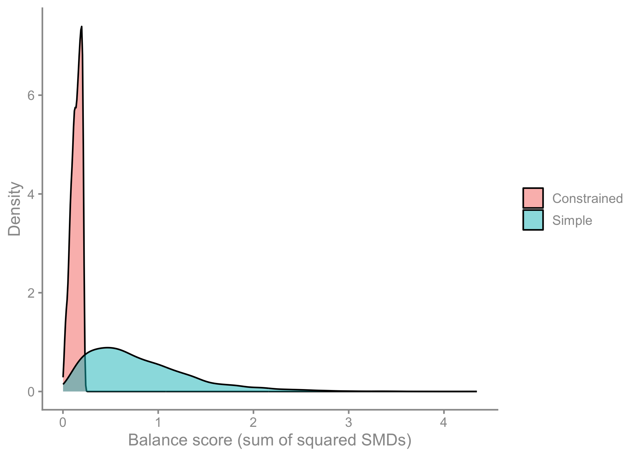
set.seed(7)simple_draws <-replicate(5000, { assignment <-sample(rep(c(1, 0), each = n_treat))balance_score(assignment, clusters_std, covars)})plot_df <-bind_rows(data.frame(score = simple_draws, method ="Simple"),data.frame(score = scores[constrained_idx], method ="Constrained"))ggplot(plot_df, aes(x = score, fill = method)) +geom_density(alpha =0.5) +labs(x ="Balance score (sum of squared SMDs)",y ="Density", fill =NULL)
The constrained distribution is concentrated near zero, whereas the simple-randomization distribution has a long right tail of poorly balanced allocations. CCR removes exactly the allocations that would have left the arms imbalanced, while still leaving a rich set to randomize among. We can quantify the improvement directly.
The constrained approach delivers a substantially lower mean balance score and, by construction, a far lower worst-case score. The practical payoff is that the analysis begins from arms comparable on the covariates we cared about, reducing reliance on model-based adjustment that a small trial can ill afford.
Finally, we check that the arms are actually comparable on the baseline covariates—the “Table 1” that opens most trial reports. For the CCR allocation, we summarize each covariate by arm and report the SMD, the conventional measure of between-arm imbalance (values below about 0.1 are generally considered well balanced).
# SMD for one covariate given an arm vectorsmd <-function(x, arm) { m1 <-mean(x[arm =="Treatment"]); m0 <-mean(x[arm =="Control"]) s1 <-var(x[arm =="Treatment"]); s0 <-var(x[arm =="Control"]) (m1 - m0) /sqrt((s1 + s0) /2)}# For a fair, reproducible comparison we contrast the best-balanced CCR# allocation with a simple-randomization allocation.best_ccr <- candidates[[ which.min(scores) ]]clusters$arm_ccr_best <-ifelse(best_ccr ==1, "Treatment", "Control")# Simple randomizationset.seed(0)a <-sample(rep(c(1, 0), each = n_treat))clusters$arm_simple <-ifelse(a ==1, "Treatment", "Control")table1 <-data.frame(Covariate = covars,`CCR: Trt`=sapply(covars, function(v) mean(clusters[[v]][clusters$arm_ccr_best =="Treatment"])),`CCR: Ctrl`=sapply(covars, function(v) mean(clusters[[v]][clusters$arm_ccr_best =="Control"])),`CCR: SMD`=sapply(covars, function(v) smd(clusters[[v]], clusters$arm_ccr_best)),`Simple: Trt`=sapply(covars, function(v) mean(clusters[[v]][clusters$arm_simple =="Treatment"])),`Simple: Ctrl`=sapply(covars, function(v) mean(clusters[[v]][clusters$arm_simple =="Control"])),`Simple: SMD`=sapply(covars, function(v) smd(clusters[[v]], clusters$arm_simple)),check.names =FALSE)table1[, -1] <-round(table1[, -1], 3)knitr::kable(table1, row.names =FALSE, digits =2)
Covariate
CCR: Trt
CCR: Ctrl
CCR: SMD
Simple: Trt
Simple: Ctrl
Simple: SMD
size
276.50
276.50
0.00
243.60
309.40
-0.97
base_rate
0.22
0.23
-0.01
0.24
0.21
0.29
ses_index
0.10
0.09
0.01
0.04
0.14
-0.12
mean_age
46.27
46.04
0.03
45.91
46.40
-0.06
The CCR arms show SMDs below 0.05 across all four covariates, whereas the simple-randomization allocation leaves several covariates imbalanced, with SMDs above 0.1.
A design caution is that the tighter the constraint, the better the balance, but the smaller the constrained randomization space and the stronger the induced dependence between allocation and covariates, which the analysis should account for (Li et al. 2016, 2017).
For trials with few clusters, CCR is a principled and practical tool, and the cvcrand package in R implements this workflow with additional features for analysis (Gallis et al. 2018; Yu et al. 2019).
References
Bailey, R. A. 1987. “Restricted Randomization: A Practical Example.”Journal of the American Statistical Association 82 (399): 712–19.
Gallis, John A, Fan Li, Hengshi Yu, and Elizabeth L Turner. 2018. “Cvcrand and Cptest: Commands for Efficient Design and Analysis of Cluster Randomized Trials Using Constrained Randomization and Permutation Tests.”The Stata Journal 18 (2): 357–78.
Hayes, Richard J., and Lawrence H. Moulton. 2017. Cluster Randomised Trials. 2nd ed. Chapman; Hall/CRC.
Ivers, Noah M., Ilana J. Halperin, Jan Barnsley, et al. 2012. “Allocation Techniques for Balance at Baseline in Cluster Randomized Trials: A Methodological Review.”Trials 13 (1): 120.
Li, Fan, Yuliya Lokhnygina, David M. Murray, Patrick J. Heagerty, and Elizabeth R. DeLong. 2016. “Evaluation of the Covariate-Constrained Randomization Design for Cluster Randomized Trials.”Statistics in Medicine 35 (10): 1565–79.
Li, Fan, Elizabeth L. Turner, Patrick J. Heagerty, David M. Murray, William M. Vollmer, and Elizabeth R. DeLong. 2017. “An Evaluation of Constrained Randomization for the Design and Analysis of Group-Randomized Trials with Binary Outcomes.”Statistics in Medicine 36 (24): 3791–806.
Moulton, Lawrence H. 2004. “Covariate-Based Constrained Randomization of Group-Randomized Trials.”Clinical Trials 1 (3): 297–305.
Murray, David M. 1998. Design and Analysis of Group-Randomized Trials. Oxford University Press.
Raab, Gillian M., and Isabella Butcher. 2001. “Balance in Cluster Randomized Trials.”Statistics in Medicine 20 (3): 351–65.
Yu, Hengshi, Fan Li, John A Gallis, and Elizabeth L Turner. 2019. Cvcrand: A Package for Covariate-Constrained Randomization and the Clustered Permutation Test for Cluster Randomized Trials.